Urban-Plumber2: UK-Kin site CLMU5 simulation

[1]:

from pyclmuapp import usp_clmu
import matplotlib.pyplot as plt
import xarray as xr
import numpy as np

[2]:

%%time
# initialize
usp = usp_clmu()

# here we use the default surface data, which is the london uk-kin data
# lat = 51.5116, lon = -0.1167
# this forcing derived from urban-plumber forcing data

usp_london = usp.run(
            case_name = "UK_Kin_default",
            SURF="surfdata.nc",
            FORCING="forcing.nc",
            RUN_STARTDATE = "2002-01-01",
            STOP_OPTION = "nyears",
            STOP_N = "12",
        )
usp_london

Copying the file forcing.nc to the /Users/user/Documents/GitHub/pyclmuapp/docs/notebooks/val/workdir/inputfolder/usp
CPU times: user 1.18 s, sys: 493 ms, total: 1.68 s
Wall time: 16min 47s

[2]:

['/Users/user/Documents/GitHub/pyclmuapp/docs/notebooks/val/workdir/outputfolder/lnd/hist/UK_Kin_default_clm0_2024-12-10_13-49-57_clm.nc']

[3]:

london_nc = usp.nc_view(usp_london[0]).sel(time=slice('2012-01-01', '2014-12-31'))
london_nc

import the observation data for comparison

[4]:

ds = xr.open_dataset('/Users/user/Documents/GitHub/pyclmuapp/inputfolder/Urban-PLUMBER/datm_files/UK-Kin/CLM1PT_data/UK-KingsCollege_clean_observations_v1.nc')
ds

[5]:

#round the time to the nearest minute
london_nc['time'] = london_nc['time'].dt.round('min')
# shift the time by 30 minutes to match the observations
london_nc['time'] = london_nc['time'] - np.timedelta64(1800, 's')
df = london_nc[['Qle','Qh','Qtau','SWup','LWup']].to_dataframe()
df_ds = ds[['Qle','Qh','Qtau','SWup','LWup']].to_dataframe()
df['Qtau'] = -df['Qtau']
df = df.merge(df_ds, on='time', suffixes=('_usp', '_obs'))
df.head(1)

[5]:

	Qle_usp	Qh_usp	Qtau_usp	SWup_usp	LWup_usp	Qle_obs	Qh_obs	Qtau_obs	SWup_obs	LWup_obs
time
2012-04-04	31.69558	16.175985	0.030384	0.0	353.656372	NaN	NaN	NaN	NaN	NaN

[6]:

%%time
# modify the surface

# tree_area_fraction=0.03
# grass_area_fraction=0.04
# bare_soil_area_fraction=0.0
# water_area_fraction=0.14
# impervious_area_fraction=0.79
# roof fraction = 0.4
# raod fraction = 0.39
# topsoil_clay_fraction=0.26
# topsoil_sand_fraction=0.45
# PCT_CLAY = 0.26
# PCT_SAND = 0.45
action = {

    #"ALB_ROOF_DIR": 0.109,
    #"ALB_ROOF_DIF": 0.109,
    "CANYON_HWR": 1.13,
    "HT_ROOF": 21.3,
    "WTLUNIT_ROOF": 0.4/(0.03+0.04+0.79),
    "WTROAD_PERV": 1 - 0.39/(0.03+0.04+0.39),
    #"ALB_IMPROAD_DIR": 0.109,
    #"ALB_IMPROAD_DIF": 0.109,
    #"ALB_PERROAD_DIR": 0.109,
    #"ALB_PERROAD_DIF": 0.109,
    #"WIND_HGT_CANYON": 50
}
usp.modify_surf(action=action, surfata_name="surface_modfied_UK_Kin.nc", mode="replace", urban_type=2)

CPU times: user 229 ms, sys: 82.7 ms, total: 311 ms
Wall time: 491 ms

[7]:

usp_london_detail = usp.run(
            case_name = "UK_Kin_detail",
            RUN_STARTDATE = "2002-01-01",
            STOP_OPTION = "nyears",
            STOP_N = "12",
            RUN_TYPE= "coldstart",
        )
usp_london_detail

[7]:

['/Users/user/Documents/GitHub/pyclmuapp/docs/notebooks/val/workdir/outputfolder/lnd/hist/UK_Kin_detail_clm0_2024-12-10_14-06-56_clm.nc']

[8]:

ludon_detail_nc = usp.nc_view(usp_london_detail[0]).sel(time=slice('2012-01-01', '2014-12-31'))
ludon_detail_nc['time'] = ludon_detail_nc['time'].dt.round('min')
ludon_detail_nc['time'] = ludon_detail_nc['time'] - np.timedelta64(1800, 's')
df_ds = ds[['Qle','Qh','Qtau','SWup','LWup']].to_dataframe()
df_detail = ludon_detail_nc[['Qle','Qh','Qtau','SWup','LWup']].to_dataframe()
df_detail['Qtau'] = -df_detail['Qtau']
df_detail = df_detail.merge(df_ds, on='time', suffixes=('_usp', '_obs'))
df_detail.head(1)

[8]:

	Qle_usp	Qh_usp	Qtau_usp	SWup_usp	LWup_usp	Qle_obs	Qh_obs	Qtau_obs	SWup_obs	LWup_obs
time
2012-04-04	35.300236	16.307856	0.029534	0.0	352.476349	NaN	NaN	NaN	NaN	NaN

[9]:

from sklearn.metrics import mean_squared_error, mean_absolute_error
import seaborn as sns
import warnings
from datetime import datetime
from scipy.stats import pearsonr
warnings.filterwarnings('ignore')

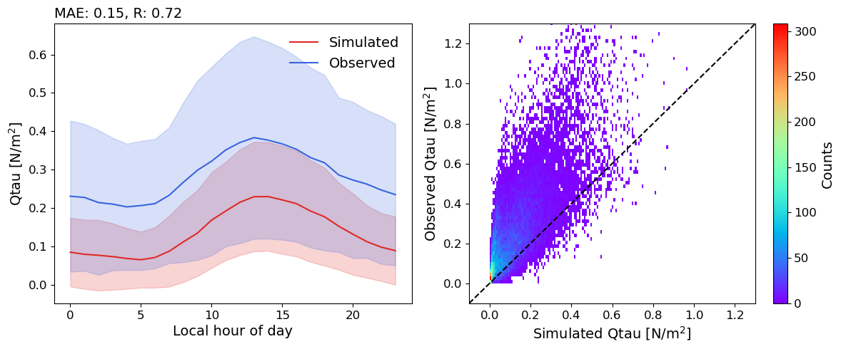
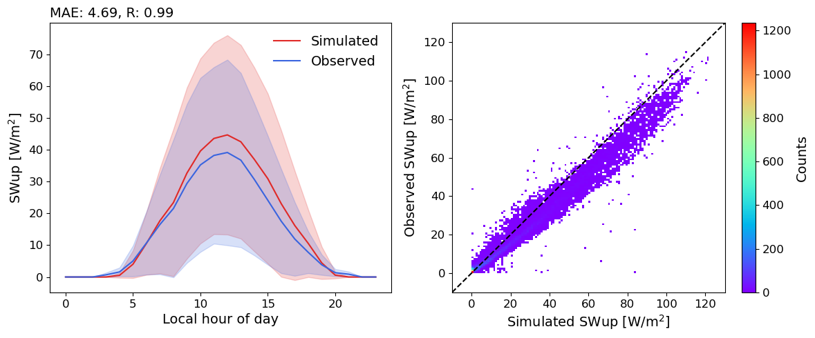
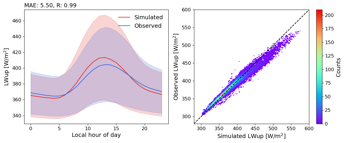
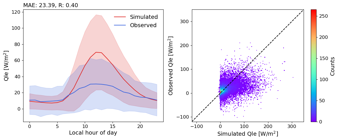
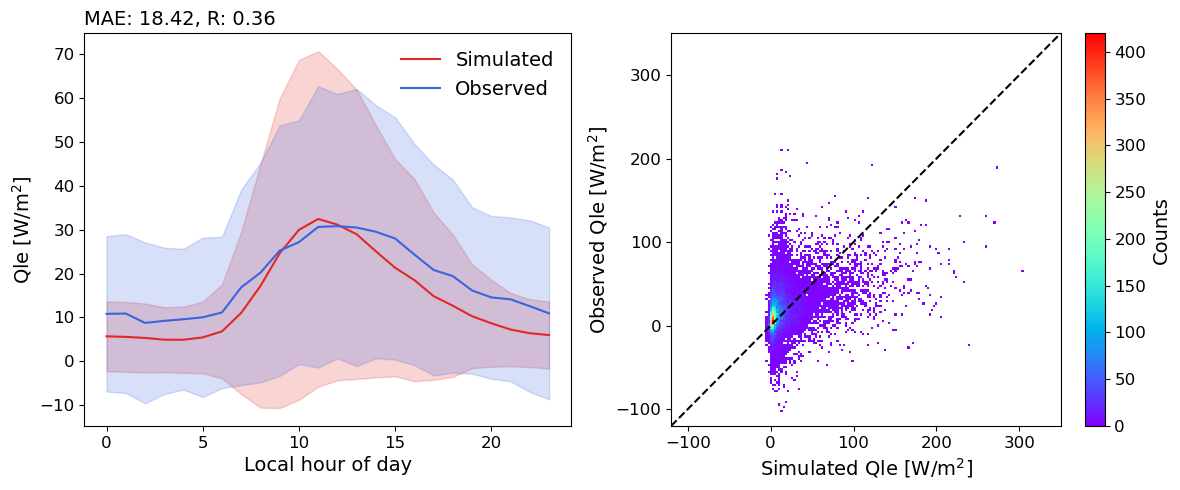
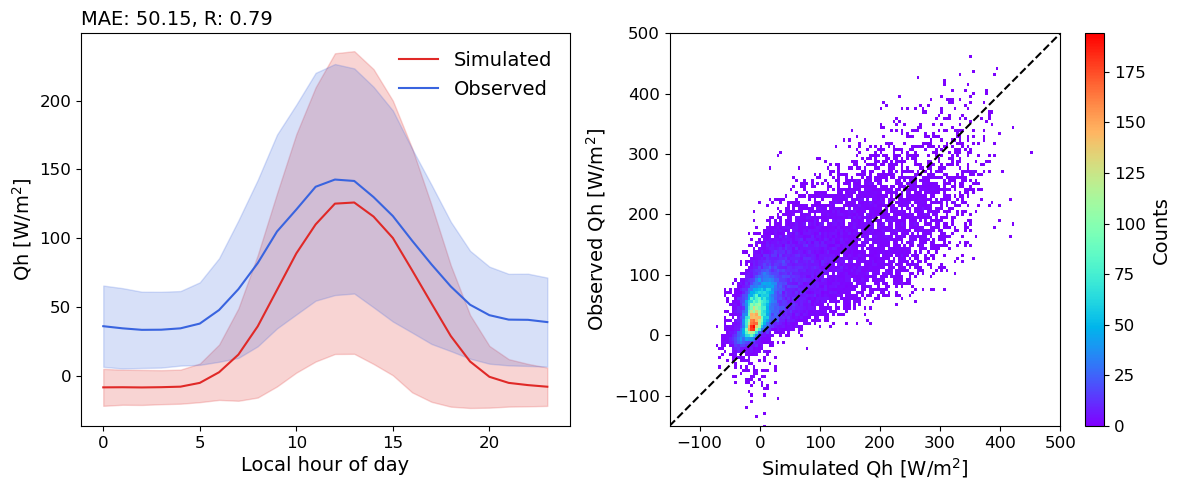
def plotting(df, save_path):
    var_list = ['SWup','LWup','Qle','Qh','Qtau']
    unit = ['W/m$\mathrm{^{2}}$', 'W/m$\mathrm{^{2}}$', 'W/m$\mathrm{^{2}}$', 'W/m$\mathrm{^{2}}$', 'N/m$\mathrm{^{2}}$']
    lim = [[-10, 130], [280, 600], [-120, 350], [-150, 500], [-0.1, 1.3]]


    for var in var_list:
        fig = plt.figure(figsize=(12, 5))

        df_plot = df[[f'{var}_usp', f'{var}_obs']].dropna()
        df_mean = df_plot[[f'{var}_usp', f'{var}_obs']].groupby(df_plot.index.hour).mean()
        df_std = df_plot[[f'{var}_usp', f'{var}_obs']].groupby(df_plot.index.hour).std()

        mae = mean_absolute_error(df_plot[f'{var}_obs'],df_plot[f'{var}_usp'])
                            #mean_absolute_percentage_error(df_plot[f'{var}_usp'], df_plot[f'{var}_obs'])#mean_squared_error(df_plot[f'{var}_usp'], df_plot[f'{var}_obs'])
        R, _ = pearsonr(df_plot[f'{var}_usp'], df_plot[f'{var}_obs'])

        ax = fig.add_subplot(1, 2, 1)

        if var == 'SWup':
            for h in range(0,24):
                if h not in df_mean.index:
                    df_mean.loc[h] = [0,0]
                    df_std.loc[h] = [0,0]
        df_mean = df_mean.sort_index()
        df_std = df_std.sort_index()

        ax.plot(df_mean.index, df_mean[f'{var}_usp'], color="#E02927", label='Simulated')
        ax.fill_between(df_mean.index, df_mean[f'{var}_usp']-df_std[f'{var}_usp'], df_mean[f'{var}_usp']+df_std[f'{var}_usp'], color="#E02927", alpha=0.2)
        ax.plot(df_mean.index, df_mean[f'{var}_obs'], color="#3964DF", label='Observed')
        ax.fill_between(df_mean.index, df_mean[f'{var}_obs']-df_std[f'{var}_obs'], df_mean[f'{var}_obs']+df_std[f'{var}_obs'], color="#3964DF", alpha=0.2)
        ax.set_ylabel(f'{var} [{unit[var_list.index(var)]}]', fontsize=14)
        ax.set_xlabel('Local hour of day', fontsize=14)
        ax.set_title(f'MAE: {mae:.2f}, R: {R:.2f}', fontsize=14, loc='left')
        ax.tick_params(axis='both', which='major', labelsize=12)
        ax.legend(frameon=False, fontsize=14)

        ax = fig.add_subplot(1, 2, 2)
        h = sns.histplot(
            x=f'{var}_usp',
            y=f'{var}_obs',
            data=df_plot,
            ax=ax,
            cmap='rainbow',
            bins=120,
            #cbar=True,
            #cbar_kws={'label': 'Counts'},
        )
        cbar = h.figure.colorbar(h.collections[0], ax=ax)
        cbar.set_label('Counts', fontsize=14)
        cbar.ax.tick_params(labelsize=12)
        ax.plot(lim[var_list.index(var)], lim[var_list.index(var)], color='black', linestyle='--')
        ax.tick_params(axis='both', which='major', labelsize=12)
        ax.set_xlabel(f'Simulated {var} [{unit[var_list.index(var)]}]', fontsize=14)
        ax.set_ylabel(f'Observed {var} [{unit[var_list.index(var)]}]',  fontsize=14)
        ax.set_xlim(lim[var_list.index(var)])
        ax.set_ylim(lim[var_list.index(var)])
        print(f'{var} MAE: {mae:.2f}')

        fig.tight_layout()
        fig.savefig(save_path + f'_{var}.pdf', dpi=300, bbox_inches='tight')
        plt.show()

[10]:

plotting(df, 'figs/CLMU5_UK-Kin_default')
plotting(df_detail, 'figs/CLMU5_UK-Kin_detail')

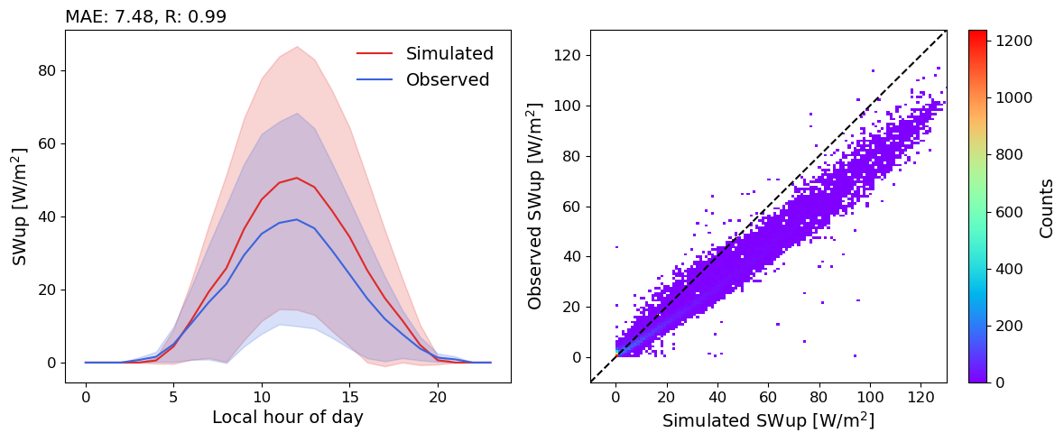
SWup MAE: 4.69

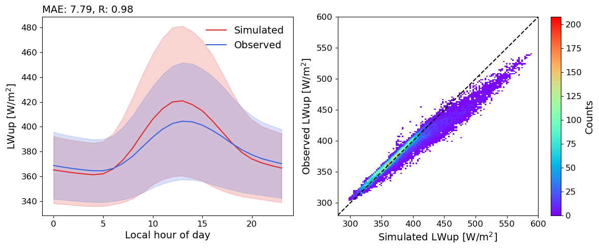
../../_images/notebooks_val_urban_plumber_usp_11_1.png

LWup MAE: 5.50

../../_images/notebooks_val_urban_plumber_usp_11_3.png

Qle MAE: 23.39

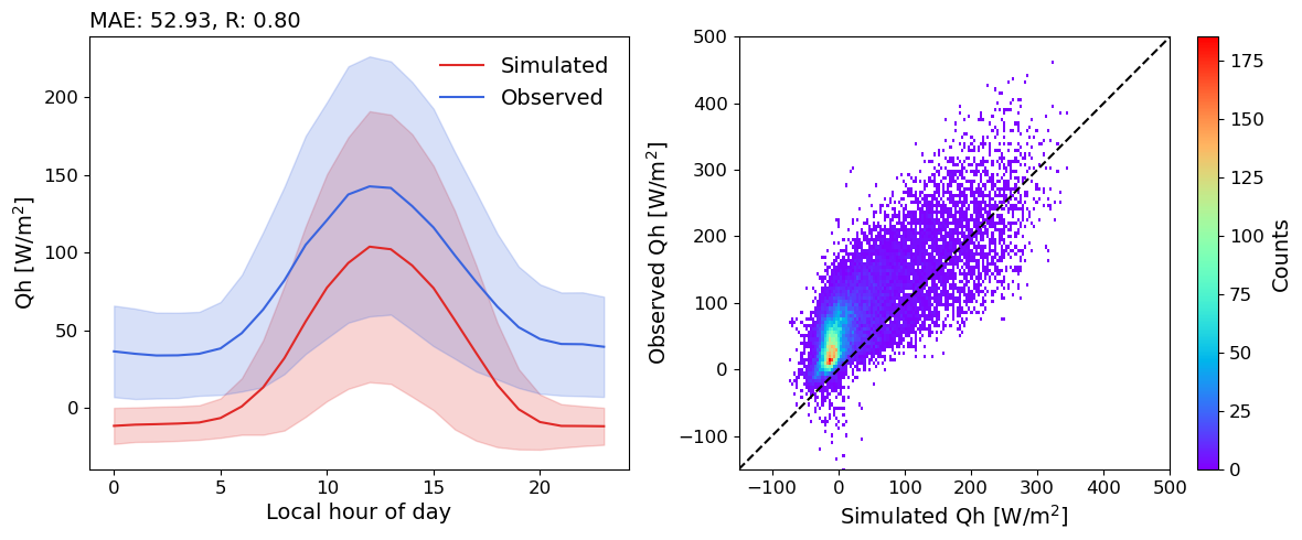
../../_images/notebooks_val_urban_plumber_usp_11_5.png

Qh MAE: 52.93

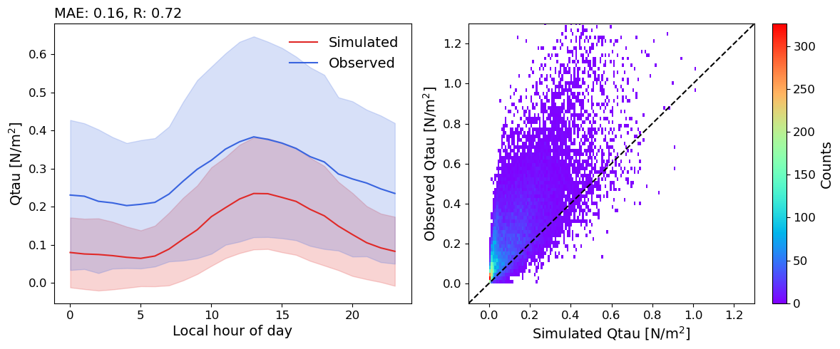
../../_images/notebooks_val_urban_plumber_usp_11_7.png

Qtau MAE: 0.16

../../_images/notebooks_val_urban_plumber_usp_11_9.png

SWup MAE: 7.48

../../_images/notebooks_val_urban_plumber_usp_11_11.png

LWup MAE: 7.79

../../_images/notebooks_val_urban_plumber_usp_11_13.png

Qle MAE: 18.42

../../_images/notebooks_val_urban_plumber_usp_11_15.png

Qh MAE: 50.15

../../_images/notebooks_val_urban_plumber_usp_11_17.png

Qtau MAE: 0.15

../../_images/notebooks_val_urban_plumber_usp_11_19.png